Brief Introduction to Physics Simulation
I’ve been working on a custom physics engine for a while now. It’s been quite a journey, and I aim to document it through a series of blog posts. In this post we’ll mostly be talking about rigid body simulation, so for now, pretend that soft bodies don’t exist. First, we’ll be going through the basic architecture of a physics engine, focusing on a 2D rigid body simulation with code examples to keep everything neat and simple.
Modeling motion
Let’s start with the most straightforward part of a physics simulation: modeling the motion of objects. For this, we’ll use the equation of motion and Newton’s second law.
F = ma

v = v + a * t
v = v + F/m * t

v is velocity
a is acceleration
t is time
This tells us that velocity of an object at a given time t. With this equation, we can compute velocity of our object given the force we want to apply and its mass. Now, to find the new position or displacement of the object, we can simply do the following:
s = s + v * t;
This is also known as Euler’s integration f(t + dt) = f(t) + f'(t) x dt. It is simply an approximation of an object’s displacement over a small interval t. Mass is an object’s resistance to changes in its linear motion. We can compute mass using an object’s density and volume.
v = width * height * depth
mass = density * volume
Here is a code example for simulating this model: Link
Angular motion (rotation)
The above equations of motion are enough for modeling linear motion, but ideally, in a simulation, we also need to model angular motion. When a force is applied to a body at a point that does not pass through its center of mass, the body will experience both linear motion and angular motion (rotation).
Before going into modeling angular motion, let’s first talk about the mass moment of inertia. The mass moment of inertia is a measure of an object’s resistance to changes in its angular motion, which depends on both the mass and how the mass is distributed relative to the axis of rotation.
Every unique shape has its own mass moment of inertia, which can be computed by combining the know mass moment of inertia of simple shapes. Deriving the mass moment of inertia of different shapes is not the goal of this post, so I will just link some resources for interested readers: How to Find Mass Moment of Inertia
The moment of inertia for commonly used shapes can be found here: List of moments of inertia
3D objects will have three axis of rotation, and thus we will have moment of inertia for each of these axes: Ixx, Iyy and Izz. This is generally represented using a 3x3 matrix called inertia tensor.
Finally for we can model angular motion as,
w = w + a * t
w = w + to/I * t

w is angulary velocity
a is angular acceleration
t is delta time


// new rotation
r = r + w * t

// wrap angle around [0, 2*PI]
if (r < 0) r += 2 * Math.PI;
if (r >= 2 * Math.PI) r -= 2 * Math.PI;
Updated example with Angular motion: Link
Resolving collision
Our motion simulation works quite well, but it has a major issue: the bodies overlap upon collision. Ideally, rigid bodies (bodies that don’t deform under force) do not overlap on collision, they exert forces on each other and may lose some energy due to friction and restitution. To address this, we first need to detect collision and then resolve them. The entire process of detecting and resolving collision can be divided into four majour stages.
- Broadphase
- Narrowphase
- Constraints
- Solver
Broadphase
In this stage, we compute a list of possibly colliding shape pairs. Possibly colliding means we don’t actually compute the precise contact points, rather determine whether a collision is possible. This can be done in a number of ways. The most widely used method involves using bounding volumes, usually an AABB (Axis Aligned Bounding Box) along with a space-partitioning structure, typically a binary tree BVH (Bounding Volume Hierarchy). Since directly computing contact between two shapes can be very expensive, the broadphase helps us avoid unnecessary computations for objects that obviously cannot collide. By using simple bounding volumes and specialized structures to keep track of those volumes broadphase checks become relatively inexpensive.
For our simple JS example, we can get away with hash grids. A hash grid is a straightforward space-partitioning structure in which the space is divided into an n × m grid, and for each cell, we keep track of the objects that intersect with it. If you are interested in implementing BVH, you might want to check out ErinCatto’s DynamicBVH slides.
Narrowphase
After we get a list of possibly colliding pairs through broadphase, we need to perform the actual collision tests between the shapes. This stage is relatively straight forward for basic shapes like spheres, but for some slightly complex shapes such as boxes, convex hulls or meshes, we’ll need to employ a combination some well-documented algorithms like SAT (Separating Axis Theorem) and GJK (Gilbert–Johnson–Keerthi) with EPA (Expanding Polytope Algorithm).
Narrowphase generates contact information such as contact points, contact normals, penetration depth, which we’ll need to resolve the contact.
Resources for these algorithms:
- GJK: Implementing GJK
- SAT: SAT for OOBB
For our small JS example, we are only using circles, and computing contact between two circles is fairly trivial.
// C1 and C2 be two possibly colliding circles
// r1 is radius of C1, r2 is radius of C2

d = distance(C1, C2);

if (d > r1 + r2) => no collision

normal = (C2 - C1) / d
point = C1 + normal * r1
penetration = (r1 + r2) - d;
Constraints
We can resolve the collision (separate the penetrating shapes) based on the information generated by the narrow phase. One way to solve collisions is through contact constraints. Constraints are limitations on the body’s degrees of freedom—a set of rules that dictate how a body can move. We can model constraints with an equation of the form C = 0, where C is our constraint that must equal zero; otherwise, the constraint fails. For example, if C represents the position of a body, C = 0 means that the position of the body should always remain at zero (essentially setting the position to zero every frame). Conversely, a constraint C greater than 0 indicates that C should be greater than zero.
Constraints allow us to model rules that control the behavior of the physics simulation. They can also be used to simulate various things, such as collision responses, joints, and springs.
For our example, let’s implement a simple ground constraint (objects shouldn’t fall off the ground). We can define our ground as y = 200, so our ground constraint will be y greater than 200.
if((pos.y - radius) <= 200) { // if the constraint is violated
    const bias = (200 - (pos.y - radius));
    pos.y += bias; // correct the positional error
    velocity.y = 0; // remove y velocity
}
Solver
A solver is essentially a piece of logic that resolves constraints so that they remain valid. The two popular ways to solve constraints are by addressing positions (as in the example above) or solving velocities. While position constraints work, they are not particularly physically accurate.
For our contacts, we will focus on velocity constraints. Velocity constraints are essentially the first derivative of the position constraint (i.e., C’ = 0). When solving velocity constraints, we will apply a small amount of impulses to the bodies until the constraint is satisfied (also known as impulse solvers).
Since impulse solvers address continuous dynamics using discrete time steps, we need to solve them iteratively. Each iteration applies small impulses to correct the velocities of the bodies until the constraints are satisfied. As with most numerical methods, increasing the number of iterations generally leads to a more refined solution, although there are diminishing returns after a certain point. A physics simulation might involve multiple constraint solvers for different types of constraints. Before diving into contact constraints, let’s go through the formulas we’ll use to compute the impulses. We already have the direction for our impulse (the contact normal); now all we need to compute is the coefficient of impulse. (magnitude).
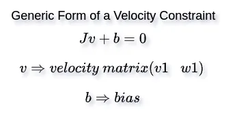
Given a velocity constraint Jv + b = 0, we can compute the coefficient of impulse as:
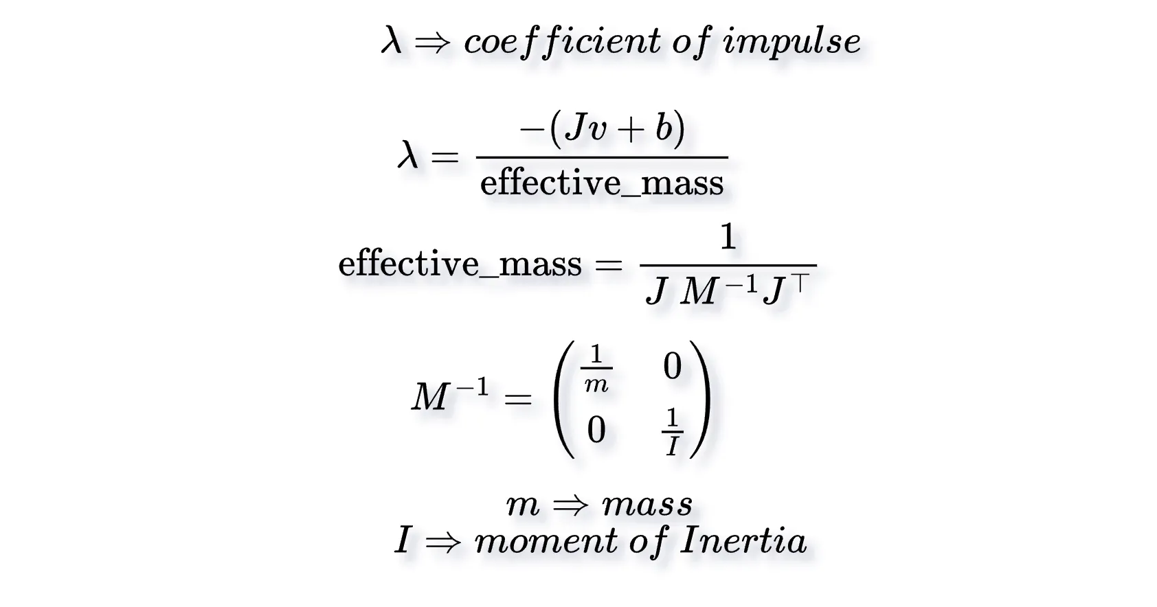
Since solving for velocities alone will not produce enough impulse to achieve the desired outcome, we can slightly boost the impulse using a bias b (e.g., penetration depth for contacts).
Contact Constraint
Now, let’s model our contact in terms of velocity constraint: (relative_velocity).n >= 0 (relative velocity projected onto the contact normal).
rv = V2 - V1 // relative velocity

jv = dot(rv, n) // n is contact normal

if(jv < 0) => bodies moving closer to each other
if(jv > 0) => bodies moving apart from each other
if(jv = 0) => no change in the movement

b = -penetration / dt (computed in Narrowphase)

l = -(jv + b) / eff_mass
impulse = l * contact_normal
But how do we computed the effective mass?
To find the effective mass, we can just plug rv.n = 0 into the generic form Jv + b = 0.
Jv = rv.n; // dot(rv, n)
Jv = (V2 - V1).n;

Jv = (v2 + w2 x c1).n - (v1 + w1 x c2).n  // x - cross product
// c1 = (contact_point - pos_a)
// c2 = (contact_point - pos_b)
// v1, w1 = velocities of body a
// v2, w2 = velocities of body b
// v = [v1 w1 v2 w2]
With this, we can now solve for J, resulting in: J = [-n -(c1 x n) n (c2 x n)]. Finally, using the effective mass equation above we can compute our effective mass as:
eff_mass = inv_m1 + dot(inv_I1 * c1n, c1n) + inv_m2 + dot(inv_I2 * c2n, c2n)

c1n = c1 x n // x - cross product
c2n = c2 x n
Applying the impulse:
v += impulse / mass
w += cross(point - centroid, impulse) / I
Clamping impulse
When our impulse is negative, it will pull two bodies towards each other instead of pushing them apart, so we’ll need to clamp our impulse. We will go with clamping method suggested by Erin Catto.
l = -(jv + b) / eff_mass

// clamping
old_l = accumulated_l
accumulated_l = max(0, old_l + l)
l = accumulated_l - old_l
Bias smoothing
If we add the bias b as it is, it will immediately correct the positional error induced by the collision. This is usually not desirable, as we would prefer our bodies to correct themselves smoothly over multiple frames. We can dampen our bias with a smoothing factor to achieve this. This is also known as Baumgarte stabilization.
bias = -0.3 * (penetration / dt); // 0.3 is our smoothing factor
Friction constraint
Solving for friction is similar to solving for contacts; instead of addressing the contact along the contact normal, we will resolve it along the tangent to the contact normal.
tangent = [normal.y, normal.x] // perpendicular to the normal

rv = V2 - V1; // relative velocity

jv = dot(rv, tangent)
l = -jv / eff_mass
impulse = l * tangent
Since we are only solving for friction, we won’t need any bias term. Additionally, the clamping logic for friction is slightly different:
max_firction = friction * total_l // total_l is normal impulse
f_old_l = f_total_l
f_total_l = clamp(f_total_l + l, -max_friction, max_friction)
f_l = f_toal_l - f_old_l;
Warm starting
Warm starting is an optimization technique that can lead to better convergence for our solvers. This involves persisting the solver output (accumulated coefficient of impulse) across multiple frames. Warm starting can facilitate proper stable stacking of objects in the simulation.
Wrap up
This article has covered important steps for creating a simple physics simulation, starting with modeling linear and angular motion we explored broadphase and narrowphase collision detection, as well as methods for resolving collisions and handling friction. While these concepts provide a good starting point, there are many more techniques we can apply to enhance the simulation further. The same principles apply to 3D physics, with the addition of a third axis, making rotations a bit different since we’ll have three rotation axes to consider.